Note
Click here to download the full example code
Image registration
Demonstration of image registration using optical flow.
By definition, the optical flow is the vector field (u, v) verifying I1(x+u, y+v) = I0(x, y). It can then be used for registeration by image warping.
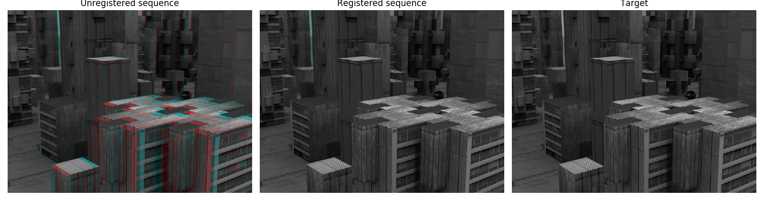
To display registration results, an RGB image is constructed by assining the result of the registration to the red channel and the target image to the green and blue channels. A perfect registration results in a gray level image while misregistred pixels appear colored in the constructed RGB image.
import numpy as np
import matplotlib.pyplot as plt
from skimage.transform import warp

import pyimof

# --- Loaf the Urban2 sequence

I0, I1 = pyimof.data.urban2()

# --- Estimate the optical flow

u, v = pyimof.solvers.tvl1(I0, I1)

# --- Use the estimated optical flow for registeration

nl, nc = I0.shape

y, x = np.meshgrid(np.arange(nl), np.arange(nc), indexing='ij')

wI1 = warp(I1, np.array([y+v, x+u]), mode='nearest')

# build an RGB image with the unregistered sequence
seq_im = np.zeros((nl, nc, 3))
seq_im[..., 0] = I1
seq_im[..., 1] = I0
seq_im[..., 2] = I0

# build an RGB image with the registered sequence
reg_im = np.zeros((nl, nc, 3))
reg_im[..., 0] = wI1
reg_im[..., 1] = I0
reg_im[..., 2] = I0

# build an RGB image with the registered sequence
target_im = np.zeros((nl, nc, 3))
target_im[..., 0] = I0
target_im[..., 1] = I0
target_im[..., 2] = I0

# --- Show the result

fig = plt.figure(figsize=(15, 4))
ax0, ax1, ax2 = fig.subplots(1, 3, True)

ax0.imshow(seq_im)
ax0.set_title("Unregistered sequence")
ax0.set_axis_off()

ax1.imshow(reg_im)
ax1.set_title("Registered sequence")
ax1.set_axis_off()

ax2.imshow(target_im)
ax2.set_title("Target")
ax2.set_axis_off()

fig.tight_layout()
plt.show()
Total running time of the script: ( 0 minutes 5.138 seconds)
